David PS

How can we access to solar data? to answer that question we need first to know what we really want to do. Many times as a student you are given an event to study, so you know the date and time of that particular event. However, other times you are interested in finding events with particular characteristics or properties.

For the first case you want to download the data from that particular event from one of the data archives available (for example in solar observations you can use virtual solar observatory, science data center, …). Nevertheless, it’s useful to know how the sun look at that particular time. You may think you are studying some quiet sun when in fact there must be a lot of things going on. For that the easiest tools to use are SolarMonitor and HelioViewer.

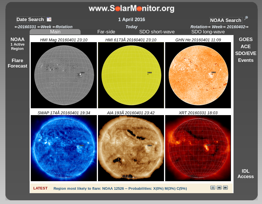
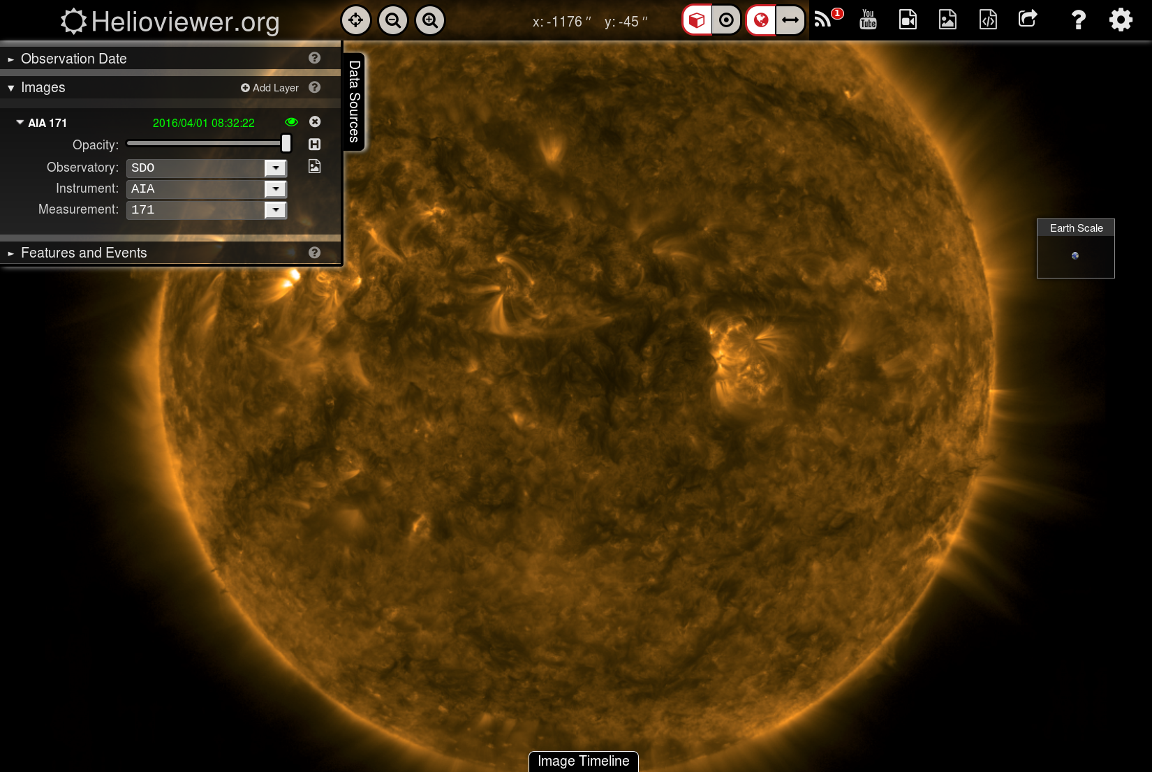
In both pages you can browse through images of the sun, but they offer different functionalities. Be free and investigate yourself what you can do with it.

On the other hand, if you want to study an event by its characteristics, and you don’t know when an event like that happened, then you need to search in catalogues of that type of events. For example, you may be interested in Coronal Mass Ejections (CMEs), and there are few catalogues of these (CaCTUS, CDAW, SEEDS, CORIMP, …), with a position angle larger than 90º. However, in these websites you can just see a table with numbers, and you don’t have an easy way to find which events have such property. Here is where tools like the HELiophysics Integrated Observatory(HELIO) and the Heliophysics Events Knowledgebase(HEK) become very useful. Below I show an example on how to work with the different services available through HELIO, but some of these steps are also possible to do through HEK.

HELIO offers different entry points, you can either access through the main front-end which provides a common interface to all the services, through each service individually or by its clients (on IDL and Python). Let’s take a look at the first two:

HELIO front end

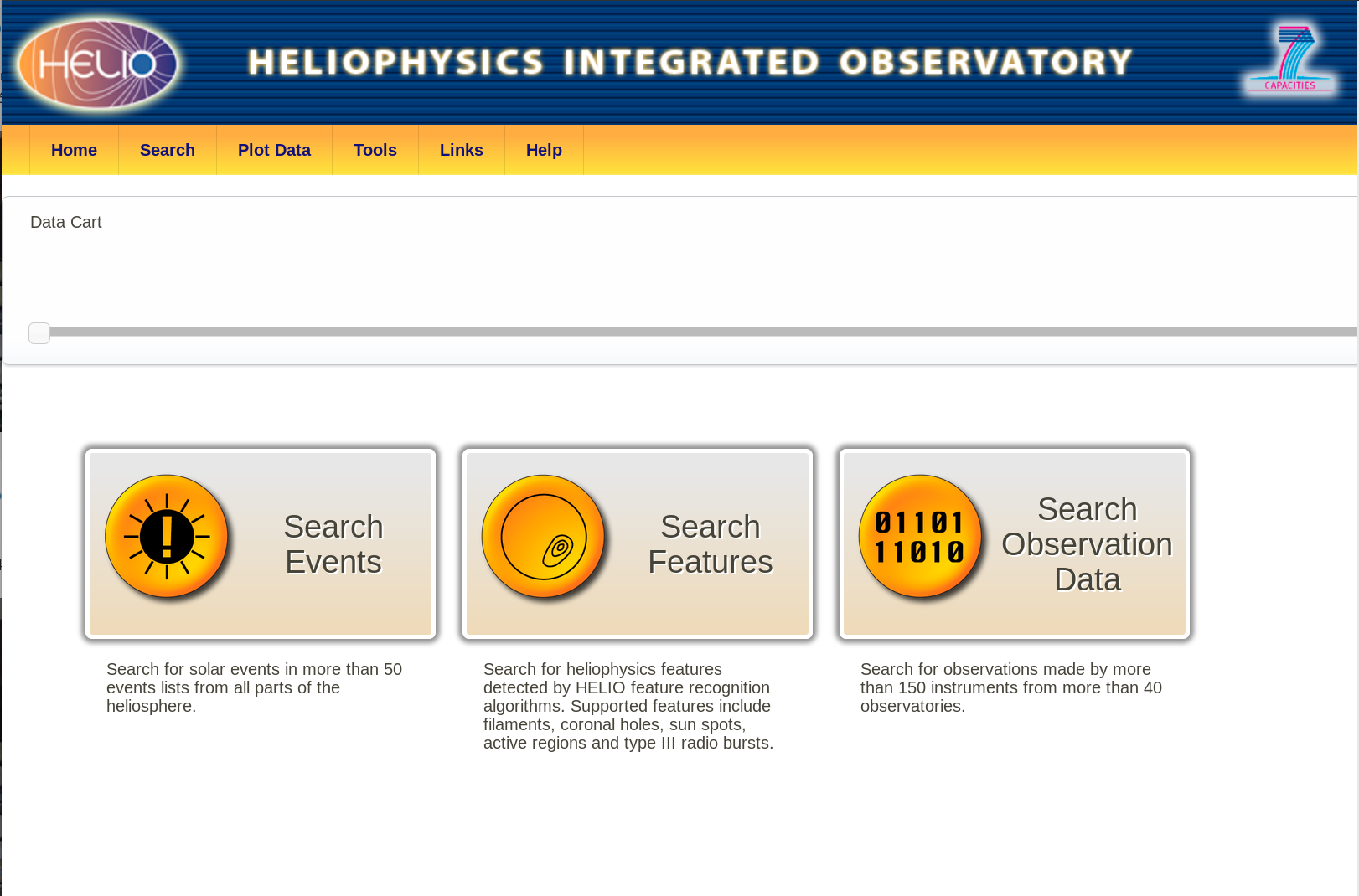
Let’s start searching for solar flares, happening between x and y. First we go to the main user interface and click on Search Events. Clicking in the empty boxes next to the clock and the event icons we’ve get a menu to select the time and the events.

Search for Flares

Set the time to be between: 2011-02-14 and 2011-03-14, and select the GOES Soft X-ray Flare List event catalogue. Clicking on submit will execute the query and return the results in a table below. That table can be sorted by any of the columns, click twice on xray_class to sort them in descending order by X-ray class.

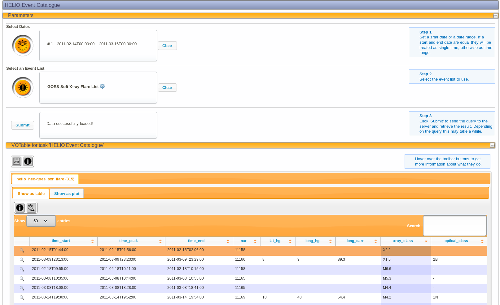
The magnifier glass placed at the left of each entry allows you to run some small programs that generates plots for understanding the situation of the sun in a plus/minus time that you can change. The default time range is set to +/- 6 hours of the starting and end time of the event.

Select the events you are interested, for example the strongest two flares of that month, by clicking on top of them (they are selected if they are in orange). Clicking the stopwatch icon just above the table extracts the times of these two events, and save them in your data cart to use it in other queries. It’s a good practice to name the extracted time, so you can differentiate it from others, to do so just write in the Name field before clicking Ok. (you can also edit the data cart afterwards)

Searching for CMEs

After selecting a flare we are interested to see if such flare produced a CME. Most of the CMEs catalogue detect them when they appear in SoHO/LASCO C2 (i.e. 2 solar radii). So, we are going to drag and drop the flare times from the data cart to the time selection icon in the same page, and click in the box to edit these times to +8 hours of the end date. 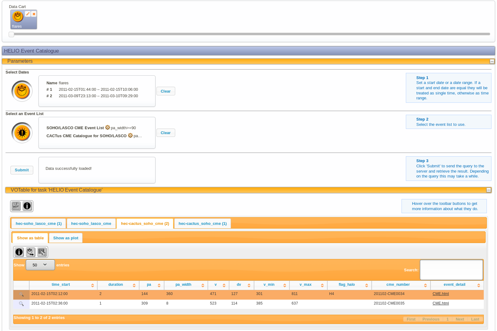Next, click in the event list box and unselect the GOES Soft X-ray Flare List by clicking in the x next to the selection. Tick CME above and choose the following catalogues: SOHO/LASCO CME Event List and CACTus CME Catalogue for SOHO/LASCO from the list. Before clicking Ok, click on the settings wheel next to the selected catalogues. This allows you to make a query based not just in a particular time range but also in the characteristics included in the catalogue. Let’s choose pa__width >= 90. This mean asks for these CMEs that show a width on the plane of sky larger than 90 degrees. Notice that once these conditions are set, the settings wheel becomes orange. Click submit.

This query produces now 4 tables, that you can see as four tabs: 2 time ranges x 2 CMEs lists. In this case, both catalogues show one event in the time ranges selected and with the condition imposed. In the last column of the CACTUS output it shows a link which directs you to their page for that event that includes a running difference video of the detected CME. As you can see some of the values between both catalogues do not match, and that’s OK. Each CME catalogue (or any other event or feature) have their own definition of what is a CME and how to measure their properties. If you are going to use these results for your research you should inform yourself on how they work and what caveats they have.

Finding the CME path

To continue with the exercise let’s save the time of the CME detected by CACTUS on 2011-02-15T02:12:00 as done previously with the flares (but this time name the extracted time as CME). Take a note too on the velocity measured by the catalogue and its error.

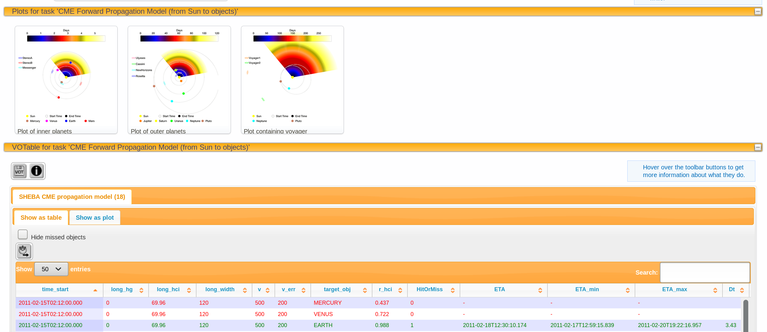
Now that we have a flare and a halo CME, we want to know when it will be seen on Earth. In the Tools menu above there’s an option for Coronal Mass Ejections (CME) Forward PM, drag the previously saved CME time and click in the select parameters box to input the “properties” of the CME. The longitude is not known (that particular flare does not include that information) but because the CME is a full 360 Halo we can assume it was launched from the centre of the solar disk (i.e. 0). The longitudinal width is something unknown with a single point of view, but 120 is a good value to see what else it hits besides Earth. For the speed and its error we can write what we got from the catalogue (500 +/- 200).

The output of this query is very similar than the one from the catalogues with a couple of extra additions, first you get three images for the progression of the CME through the solar system at three different zoom levels. The table with the results it shows in green the planets or spacecraft that may have been hit and in which time range. We’ve got that the Earth should see the CME between the 17th and 20th of February (ETA min and max respectively). You can save these times as done before, however you will need to edit them manually as it doesn’t save the estimated time of arrival but the starting time of the CME.

Confirming Earth impact

Let’s check whether ACE has seen something in that time range. Click in the Plot Data menu in the top bar, and choose ACE timeline. As usual, drag and drop the time obtained from the propagation model and click submit.

if that doesn’t work access to that service through its website and input manually the dates and choose ACE.

In case that this fails too, you can obtain a similar plot from cdaweb selecting ACE, Plasma solar wind and AC_H2_SWE.

The resulting plot effectively shows that there is an increase of solar wind speed and large variations of the magnetic field.

Cross checking with different catalogues

To get a confirmation that such flare, CME and increase in solar wind speed are connected we can go back to Search Events and clear the previous time and list selections and put the Earth time and select the Interplanetary Shock List from SOHO/CELIAS-PM as a catalogue. You will see that this catalogue includes the event we have just connected as it was detected by SoHO/CELIAS.

Searching and downloading data

To end this preliminary analysis and carry on with a more in depth study we have just to the observed data. We’ve got already the dates of interest for each of the sections, but we still need the instruments. You may known already some instruments that you may want to use, but HELIO helps you to find instruments based in the capabilities you want. Let’s search such instruments in the Search/Instruments by capability.

Flare data

For the first bit, the time when the flare starts we want to see the solar disk (the magnetic field and the corona) and also the xray flux. To do so we drag and drop the time to the time field, submit the query and filter it by the different properties. For the images on disk we click Sun on ‘Observing domain 1’, disk/inr. corona on ‘Observing domain 2’, remote from ‘instrument type’ and EUV for ‘observable entity’ to select the images at corona temperatures or magnetograph in ‘keywords’ to select the magnetic field in the solar surface. Filtering as such the list we could select SDO: Atmospheric Imaging Assembly (EUV) (AIA-EUV) and Hinode: Solar Optical Telescope/ Filter vector-magnetogram (SOT/FG) for the magnetic field. Once the instruments have been selected, you can click in the extract instruments button and get them in your data cart.

CME

For the CME we can repeat the previous steps, but instead selecting disk/inr. corona we want this time to select outer corona so we can choose coronagraph like SOHO: Large Angle Spectroscopic Coronagraph (LASCO) and MLSO: Coronagraph, Mk IV (MK4).

Near Earth environment

Similarly for the solar wind near Earth, selecting Earth on ‘observing domain 1’, in-situ for ‘Instrument type’ and magnetometer for ‘keywords’ we get instruments like ACE: Magnetic Field Experiment (MAG) and Wind: Magnetic Fields Instrument (MFI)

Downloading what’s available

Our data card should have three times selections and three instrument selections. These can be used now to search the data available under Search/Observation Data. Searching each time range with its particular instrument selections we can get the links to download the data. Once you obtain the list of files you want, the easiest way to download it is following the instructions you find when clicking in the export table button above the result table.

et voila, you’ve got now all the data from the Sun to Earth to study this particular event.

Note, that you may have selected some instruments which observes just a portion of the sun. This tools doesn’t assure you they are observing the bits you are interested in.

HELIO sql (super powers)

In HELIO you can use SQL lenguage to extract the properties in a more practical way. You can learn the basics of the language online. Below I show some simple examples on how to use it for query the event catalogues available in HELIO (HEC). Go to the Free SQL search page available from the bottom of the HEC page.

The default query that appears:

SELECT * FROM goes_sxr_flare LIMIT 10

asks to print all the columns (SELECT *) from the GOES soft x-rays flare list (called goes_sxr_flare) and limit the results to one 10 entries.

If we want to obtain a list like before, where we were looking for all the flares in a year since 2011-02-14T00:00:00 to 2012-02-13 23:59:59 then we modify the query as:

SELECT * FROM goes_sxr_flare 
         WHERE time_start>='2011-02-14 00:00:00' AND time_start<='2012-02-13 23:59:59'

if additionally we want just the ones of type X we can add:

SELECT * FROM goes_sxr_flare 
          WHERE time_start>='2011-02-14 00:00:00' AND 
                time_start<='2012-02-13 23:59:59' AND 
                xray_class LIKE 'X%'

finally, to order them by that column we could do:

SELECT * FROM goes_sxr_flare 
         WHERE time_start>='2011-02-14 00:00:00' AND 
               time_start<='2012-02-13 23:59:59' AND 
               xray_class LIKE 'X%' 
         ORDER BY xray_class DESC

That’s the same result we were obtaining before.

This tool allows us to do things more general, like for example to count the flares for each class during that year.

SELECT SUBSTRING(xray_class from 1 for 3) AS xray, COUNT(*) 
         FROM goes_sxr_flare 
         WHERE time_start>='2011-02-14 00:00:00' AND 
               time_start<='2012-02-13 23:59:59' 
         GROUP BY xray 
         ORDER BY xray DESC

In this query we are extracting the first three characters of the xray_class column (to account for larger than X9 flares) and group the flares found in such category and count them (COUNT(*)).

If you remove the WHERE condition in the last example you obtain the amount of flares obtained in the whole story of the catalogue.

The posibilities are almost endless, and this is just querying a single table, but you could construct queries from multiple of them at once. Check my list of handy queries to learn more about it.

Summary

I hope this has been helpful and it makes your life easier. Additional examples on how to use HELIO can be found in the screencast and the open access paper about the system.

Do not hesitate to report problems with the system or ask for help. You know where to find me.

Enjoy!

PS: Do not forget to play around with the HELIO feature catalogue which also allows you to use a visual and a SQL interface.

*PPS: Did you know you can access to this from SunPy?